Visual examples¶

Paired observations¶

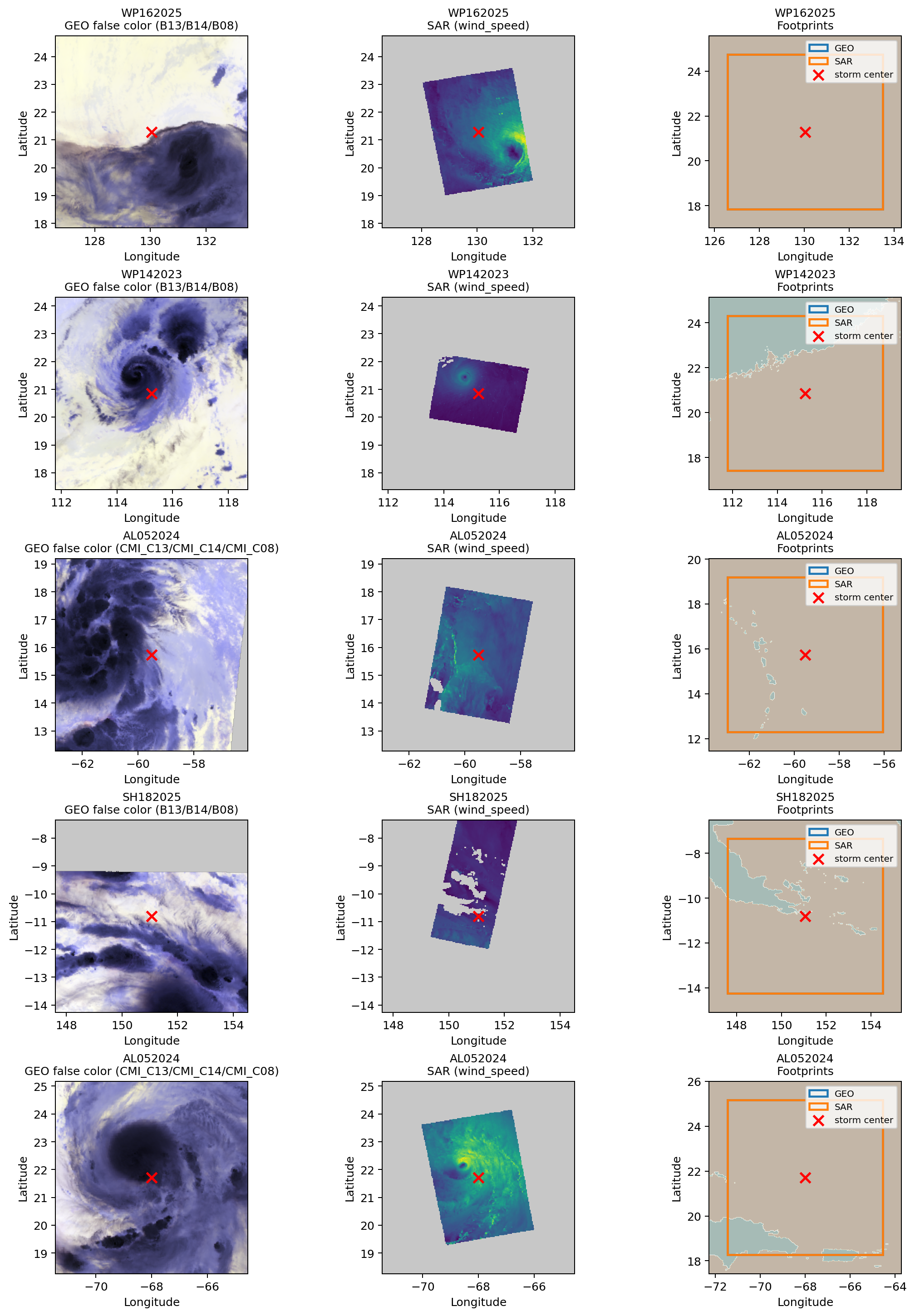
Random GEO–SAR pairs — Five random training pairs. Left: GEO false-color RGB. Middle: SAR wind speed. Right: valid footprints over an ocean/land mask. The red × is the manifest’s IBTrACS center.

The false-color view maps two infrared channels to red/green and a water-vapor channel to blue. It is a visualization, not the literal model input: the model receives all configured bands as separate normalized channels.

The footprint panel exposes the central learning challenge. GEO may cover the crop broadly while SAR is a narrower, irregular swath. target_mask prevents missing SAR pixels from becoming zero-wind labels.

W&B reconstruction panel¶

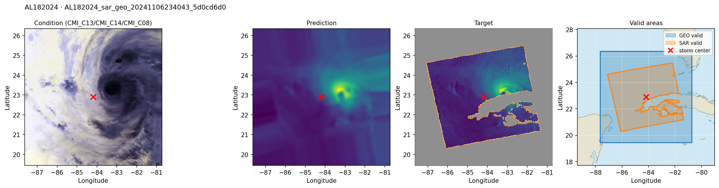
W&B reconstruction logging preview — Example condition / prediction / target panels logged from validation and a small training subset.

Current validation logging is shared by both model paths. It renders up to five georeferenced samples, labels storm and sample IDs, shades target no-data, plots the IBTrACS center, adds valid-area and ERA5 wind panels when metadata is available, caps the longest edge at 1600 pixels, and sends a compact JPEG to W&B. Diffusion panels use normalized predictions/targets; residual panels use physical m/s values. Prediction and target share a display stretch derived only from valid ground-truth pixels.

The qualitative comparison should be read alongside physical metrics. Look for:

correct storm-center placement;
low-wind eye versus high-wind eyewall contrast;
azimuthal asymmetry rather than only a smooth radial blob;
realistic radius of maximum wind;
behavior at the observed swath boundary; and
saturation or clipping artifacts.

Recreate the pair figure¶

src.utils.plotting.plot_random_geo_sar_pairs() reads the split manifest and GeoTIFF metadata:

from src.utils.plotting import plot_random_geo_sar_pairs

plot_random_geo_sar_pairs(
    "data/geotiff/geo_sar",
    split="train",
    n=5,
    seed=42,
    output_path="docs/assets/images/geo-sar-random-pairs.png",
)

The helper resolves generic condition_path/target_path first and falls back to legacy geo_path/sar_path. Band requests tolerate equivalent Bxx and Cxx names across AHI/ABI descriptions.