Dataset and access
The scientific dataset is hosted at simon-donike/geo2wf-data on Hugging Face. Its companion model repository is simon-donike/geo2wf-models. Git contains the loaders, models, and usage docs; scientific data files are stored separately.
What the release contains
The published dataset card reports 96,109 catalog samples, 14,471 observation representations, 22 source cohorts, and 18,940 scientific assets (32.9 GB in decimal units). Catalog rows span processing versions, scalar forecast sequences, paired imagery, and case-study products. They are not 96,109 independent satellite images or a single universal train/test split.
| Directory | Contents |
|---|---|
index/ | Sample, observation, asset, and storm catalogs in Parquet and CSV |
cohorts/ | Ordered source experiment manifests |
effective-cohorts/ | Loader eligibility, RI labels, and historical training membership |
assets/ | Processed GeoTIFFs, case-study NetCDFs, derived NPZ fields, and caches |
normalization/ | Fixed statistics associated with the original exports |
labels/ | Track and intensity references |
reference-results/ | Paper, case-study, and dashboard outputs |
provenance/ | Original indexes, processing metadata, and path mappings |
Consult the Hub's schema.json, release.json, and SHA256SUMS for the schema, inventory, and checksums. Optional modalities are absent when unavailable. The release includes processed training GeoTIFFs and source NetCDFs for Humberto, Kiko, and Otis; upstream raw training granules must be acquired separately to rebuild the exports. Source attribution and reuse terms are recorded in the dataset's ATTRIBUTION.md.
Browse and download
Both repositories are public and can be downloaded without an account or token. From the root of the Git checkout, use Python 3.10 or 3.11 and install the Hugging Face CLI:
The default downloads only release guides, inventories, attribution, and checksum lists from both repositories. It does not download catalog tables, imagery, or model weights. Choose a larger download explicitly:
| Command | Contents | Destination |
|---|---|---|
python3 scripts/download_artifacts.py metadata | Small metadata files from both releases | Both folders below |
python3 scripts/download_artifacts.py data | Complete dataset, including all scientific assets | downloads/data/ |
python3 scripts/download_artifacts.py models | All checkpoints, configs, provenance, and source archive | downloads/models/ |
python3 scripts/download_artifacts.py all | Complete data and model releases | Both folders |
Add --dry-run to inspect file sizes and cached status without downloading payloads, or --output-dir /path/to/storage to change the destination parent. Allow space for at least 32.9 GB of scientific assets and 1.27 GB of checkpoints, plus catalogs, provenance, source extraction, and working files. The dry run reports the complete release sizes. If interrupted, rerun the same command; the Hub client reuses completed files and its download cache.
The script pins this matching pair from the 2 October 2026 release:
| Repository | Immutable commit |
|---|---|
simon-donike/geo2wf-models | b4399d426b80698d4cf73a77c9541071a8ab3d42 |
simon-donike/geo2wf-data | 043c7f23e5f0a1fbda7034c342113664fb6aa81e |
The data commit comes from the model release's dataset-links.json. To select another release manually, use hf download with --revision <full-commit-hash> and obtain its matching data revision from that file. For example, to fetch only catalog tables for this release:
hf download simon-donike/geo2wf-data --repo-type dataset \
  --revision 043c7f23e5f0a1fbda7034c342113664fb6aa81e \
  --include 'index/*' --local-dir downloads/data
After a complete download, verify each release against its checksum list (Linux; on macOS use shasum -a 256 -c SHA256SUMS):
Partial downloads will report missing files with this full-release check. Selective dataset downloads through the release tools below verify the assets they fetch.
Use the downloads
The Hub dataset is a catalog with referenced assets. This checkout's loaders expect the local export layout, so passing downloads/data directly as data.root will not work. For released models and paper reproduction, use the matching source archive supplied with the models.
After downloading models (or all), run these commands from the Git checkout root. Extract into a new directory:
download_root="$(pwd)/downloads"
mkdir -p "$download_root/source"
tar -xzf "$download_root/models/code/conference-source.tar.gz" \
  -C "$download_root/source"
cd "$download_root/source/geo2wf"
uv sync --frozen --group dev --group docs
If you changed --output-dir, set download_root to that absolute path. The archive includes scripts/release_hub.py, scripts/conference_release.py, and catalog loaders that are separate from this Git checkout. From the extracted source, download just the paper evaluation data and run an evaluation:
uv run python scripts/release_hub.py download \
  --repo-id simon-donike/geo2wf-data \
  --revision 043c7f23e5f0a1fbda7034c342113664fb6aa81e \
  --root "$download_root/data" --profile paper-eval
uv run python scripts/conference_release.py evaluate-architecture \
  --artifact-root "$download_root/models" --catalog-root "$download_root/data" \
  --era5 with-era5 --output build/paper-results
The release downloader supports index-only, paper-eval, train, storms, and all profiles, with --cohort, --split, and --storm filters. These are different from the four simple download choices in this checkout's script. See the downloaded models/README.md, models/release/hosting/README.md, and the extracted docs/reproduction.md for training, offline use, and storm runs. For new work with this checkout, follow the local data contract and first experiment.
Inputs and targets
| Source | Channels / quantity | Use |
|---|---|---|
| GEO | ABI CMI_C07–CMI_C16 or AHI B07–B16 | Ten separate input bands |
| ERA5 | Water vapor, SST, pressure, 2 m temperature/dewpoint, 10 m u/v; derived wind speed and vorticity | Nine optional context channels |
| Geometry and solar time | Center distance, local-solar-time sine/cosine, solar zenith | Four derived input channels |
| SAR | Retrieved surface wind speed in m/s and a validity mask | Field supervision |
| IBTrACS | USA_WIND and available wind radii | Scalar supervision and storm geometry |
SAR is used during training and evaluation, not as an inference input. PMW companions can be retained by the data loader but are not required by the paper's GEO-based models. ERA5 supplies environmental context; it is not truth.
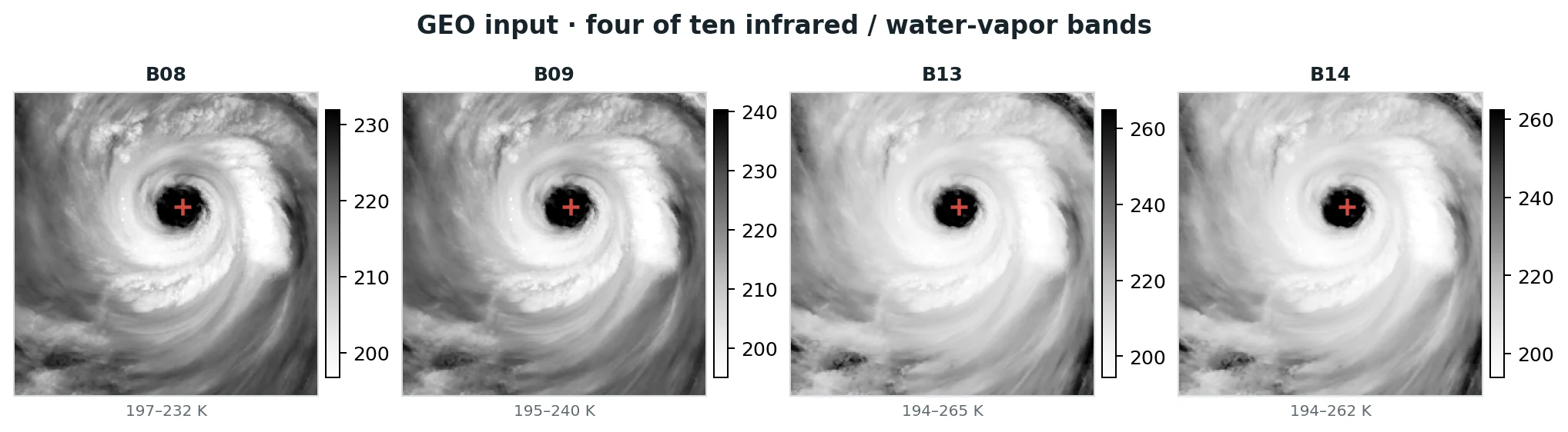
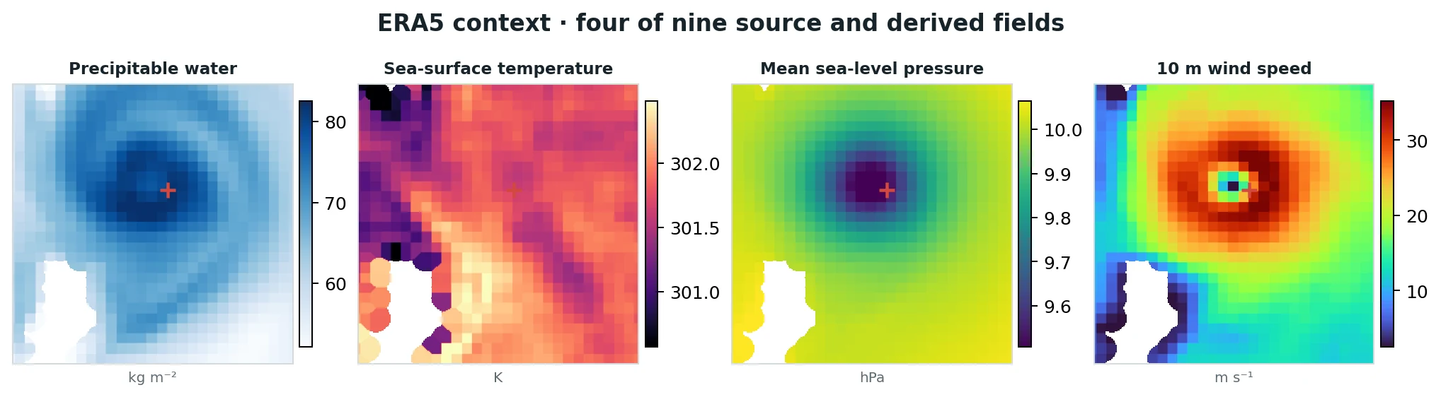
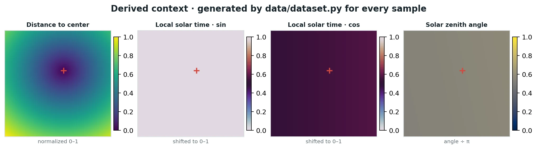
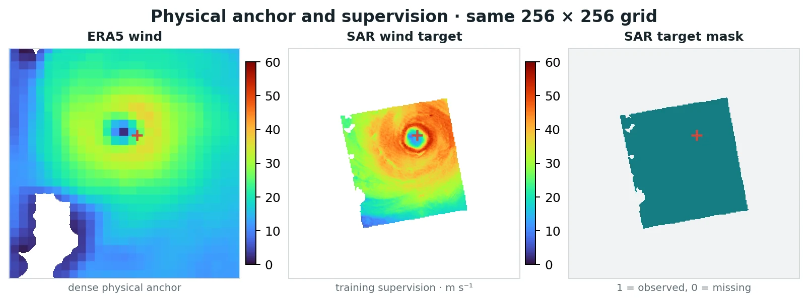
These figures show sample WP232024_sar_geo_20241030095303_bb2c52ca on its 256 × 256 export grid. Current training presets take a 192 × 192 center crop. The rasters use EPSG:4326 at 0.027° spacing; physical pixel distances vary with latitude. Figure metadata records the sources and rendering settings.
Cohorts and paper counts
The paper reports 841/232/212 train/validation/test samples from 115/34/38 storms before the additional center-valid restriction described for its supervision ablation. These counts describe the paper's processing cohort. The 1,205-row website inventory describes a different paired export, and the StormSense manifest describes dense case-study observations. Neither is the complete Hugging Face catalog.
The release preserves actual experiment membership in effective-cohorts/. Its provenance distinguishes architecture test results from latent-ablation validation results and records historical training/test overlap for an auxiliary field model. Use those records when assessing a checkpoint; do not treat the combined catalog as a newly held-out benchmark.